I participated to a project for a leading insurance company where I implemented a Record Linkage engine using Spark and its Machine Learning library, Spark ML. In this post, I will explain how we tackled this Data Science problem from a Developer’s point of view.

Use Case

The insurer has a website in France where clients like you and me can purchase an insurance for their home or car. Clients may come to this website through a quote comparison website such as LesFurets.com or LeLynx.com. When this is the case, the comparison website should be retributed for bringing a new client.

First issue is, the client might make a first quote comparison then, only a couple of weeks later, proceed with the subscription. The commission should still be paid, though. That’s why we have to compare the listings of clients – the listing from the insurer and the listing from the quote comparison website – and link records together: that’s what we call Record Linkage.

Second issue is, neither the insurer nor the comparison website are willing to provide their full listing to each other. They want to keep this confidential and, as a workaround, they provide anonymized data.

A secondary use case is when we have to find duplicates in a listing of clients. This can be done using the same engine and that explains why this problem can carry several names: Deduplication, Entity Resolution…

To come back to the first use case, we start by putting the two listings together. We end up with a dataset similar to what follows:

+---+-------+------------+----------+------------+---------+------------+
| ID|    veh|codptgar_veh|dt_nais_cp|dt_permis_cp|redmaj_cp|     formule|
+---+-------+------------+----------+------------+---------+------------+
|...|PE28221|       50000|1995-10-12|  2013-10-08|    100.0|       TIERS|
|...|FO26016|       59270|1967-01-01|  1987-02-01|    100.0|VOL_INCENDIE|
|...|FI19107|       77100|1988-09-27|  2009-09-13|    105.0|TOUS_RISQUES|
|...|RE07307|       69100|1984-08-15|  2007-04-20|     50.0|       TIERS|
|...|FO26016|       59270|1967-01-07|  1987-02-01|    105.0|TOUS_RISQUES|
+---+-------+------------+----------+------------+---------+------------+

As you can see, this dataset does not contain nominative data: the veh column holds the type of vehicle, not its license plate, the postal code is indicated in the codptgar_veh column but not the full address, etc.

Here, highlighted in red are two records that look similar. Postal codes are identical, birth date (dt_nais_cp column) is very close and so is the bonus rate (redmaj_cp), but the types of contracts are different (formule).

Prototype

A Data Scientist had implemented a prototype. It consisted of 3 steps:

Preprocessing of the data to find potential duplicates and do some Feature Engineering.
A step of manual labeling of a sample of the potential duplicates.
Machine Learning to make predictions on the rest of the records.

The Data Processing step was implemented using Spark but with a lot of SQL (parsed at runtime so you get no help from the compiler), the source code wasn’t versioned and it had no unit tests. Also, the Machine Learning part was implemented using Scikit-Learn, meaning an extra step was required to export the data from Spark and load it back into Scikit-Learn.

Obviously, my role was to industrialize the prototype and to allow it to run a larger datasets thanks to a full-Spark implementation.

Preprocessing of the data

Inputs

The input dataset is a CSV file (or 2 CSV files that we merge together) without a header:

000010;Jose;Lester;10/10/1970
000011;José;Lester;10/10/1970
000012;Tyler;Hunt;12/12/1972
000013;Tiler;Hunt;25/12/1972
000014;Patrick;Andrews;1973-12-13

CSV files are easy to read for humans but they don’t carry metadata such as what is the type of each field, what is the format of date fields, or how what processing to apply to a field.

To supplement the CSV file, we use a manually-crafted JSON file that describes all the fields and the processing to apply to each field:

{
  "tableSchemaBeforeSelection": [
    {
      "name": "ID",
      "typeField": "StringType",
      "hardJoin": false
    },
    {
      "name": "name",
      "typeField": "StringType",
      "hardJoin": true,
      "cleaning": "digitLetter",
      "listFeature": [ "scarcity" ],
      "listDistance": [ "equality", "soundLike" ]
    },
    ...

Data loading

The first step consists in loading the data, in particular the CSV file. We use the open source Spark CSV module to load the file into a Spark DataFrame. As the CSV file doesn’t carry a header, we provide the schema to the reader thanks to metadata read from the JSON file.

Also, we disable the type inference mechanism for 2 reasons:

It is not possible to provide the format for parsing dates.
Some fields could be transformed when you don’t want them to: in our case, the ID field would be detected as an integer but we want to keep it as a string.

+------+-------+-------+----------+
|    ID|   name|surname|   birthDt|
+------+-------+-------+----------+
|000010|   Jose| Lester|10/10/1970|
|000011|   José| Lester|10/10/1970|
|000012|  Tyler|   Hunt|12/12/1972|
|000013|  Tiler|   Hunt|25/12/1972|
|000014|Patrick|Andrews|1970-10-10|
+------+-------+-------+----------+

Data cleansing

The data cleansing step is pretty straightforward. We parse numbers, booleans and dates so as to have primitive types instead of strings. We also convert all strings to lowercase and remove accentuated characters.

This step is implemented with User Defined Functions implemented in Scala.

Notice, in the following example, how an invalid date was turned into a null value.

+------+-------+-------+----------+
|    ID|   name|surname|   birthDt|
+------+-------+-------+----------+
|000010|   jose| lester|1970-10-10|
|000011|   jose| lester|1970-10-10|
|000012|  tyler|   hunt|1972-12-12|
|000013|  tiler|   hunt|1972-12-25|
|000014|patrick|andrews|      null|
+------+-------+-------+----------+

Feature calculation

Then comes the step of feature calculation where we add new columns calculated from existing columns.

In this example, the BMencoded_name column is the phonetics calculated from the name column. We have used the Beider Morse encoding from the Apache Commons Codec library but we could instead have used the Double Metaphone encoding.

+------+-------+-------+----------+--------------------+
|    ID|   name|surname|   birthDt|      BMencoded_name|
+------+-------+-------+----------+--------------------+
|000010|   jose| lester|1970-10-10|ios|iosi|ioz|iozi...|
|000011|   jose| lester|1970-10-10|ios|iosi|ioz|iozi...|
|000012|  tyler|   hunt|1972-12-12|               tilir|
|000013|  tiler|   hunt|1972-12-25|    tQlir|tili|tilir|
|000014|patrick|andrews|      null|pYtrQk|pYtrik|pat...|
+------+-------+-------+----------+--------------------+

Find potential duplicates

Then comes what is probably the most important – and also the most computationally expensive – step: finding records that are potential matches. The goal is to find records that look similar without necessarily being identical field by field.

This step is basically an inner join of the table with itself. The join condition is very specific: we chose to match records that have at least 2 fields that are equal. This is broad enough so that catch records with several differences, while at the same time selective enough to avoid a cartesian product (cartesian products should be avoided at all costs).

+------+------+---------+...+------+------+---------+...
|  ID_1|name_1|surname_1|...|  ID_2|name_2|surname_2|...
+------+------+---------+...+------+------+---------+...
|000010|  jose|   lester|...|000011|  jose|   lester|...
|000012| tyler|     hunt|...|000013| tiler|     hunt|...
+------+------+---------+...+------+------+---------+...

Distance calculation

Now that we have found potential duplicates, we need to calculate features for them. We use several methods to score the proximity of the fields: for strings, we can determine the equality or calculate the Levenshtein distance, while, for dates, we may calculate the difference in days.

+------+...+------+...+-------------+--------------+...+----------------+
|  ID_1|...|  ID_2|...|equality_name|soundLike_name|...|dateDiff_birthDt|
+------+...+------+...+-------------+--------------+...+----------------+
|000010|...|000011|...|          0.0|           0.0|...|             0.0|
|000012|...|000013|...|          1.0|           0.0|...|            13.0|
+------+...+------+...+-------------+--------------+...+----------------+

Standardization / vectorization

The final data processing step consists in standardizing the features and vectorizing them. This is standard so that we can apply a Machine Learning algorithm.

Notice that we create 2 vectors (distances and other_features), not just one. This is to allow us to filter the potential duplicates that have a distance we consider to be too high.

+------+------+---------+----------+------+------+---------+----------+------------+--------------+
|  ID_1|name_1|surname_1| birthDt_1|  ID_2|name_2|surname_2| birthDt_2|   distances|other_features|
+------+------+---------+----------+------+------+---------+----------+------------+--------------+
|000010|  jose|   lester|1970-10-10|000011|  jose|   lester|1970-10-10|[0.0,0.0,...|  [2.0,2.0,...|
|000012| tyler|     hunt|1972-12-12|000013| tiler|     hunt|1972-12-25|[1.0,1.0,...|  [1.0,2.0,...|
+------+------+---------+----------+------+------+---------+----------+------------+--------------+

Spark – From SQL to DataFrames

The prototype implementation was generating a lot of SQL requests then interpreted by Spark. While plain SQL requests can be easy to read for humans, they become hard to understand and to maintain when they are generated, especially when User Defined Functions come into play. Here is an example of code that was written to generate a SQL request:

val cleaningRequest = tableSchema.map(x => {
  x.CleaningFuction match {
    case (Some(a), _) => a + "(" + x.name + ") as " + x.name
    case _ => x.name
  }
}).mkString(", ")

val cleanedTable = sqlContext.sql("select " + cleaningRequest + " from " + tableName)
cleanedTable.registerTempTable(schema.tableName + "_cleaned")

We can see that the SQL request is broken down into many parts and it’s hard to see what processing is being done.

We rewrote that part to rely only on DataFrame primitives. That way, more work is done by the compiler and less is done at runtime.

val cleanedDF = tableSchema.filter(_.cleaning.isDefined).foldLeft(df) {
  case (df, field) =>
    val udf: UserDefinedFunction = ... // get the cleaning UDF
    
    df.withColumn(field.name + "_cleaned", udf.apply(df(field.name)))
      .drop(field.name)
      .withColumnRenamed(field.name + "_cleaned", field.name)
}

Unit testing

Because of the rewrite of the code from SQL to DataFrames, most of the code of the prototype was refactored. This introduced heavy changes while we needed to secure that the functionality would remain the same. To make sure this would be the case, we wrote unit tests to cover all the data processing operations.

Because we were writing code in Scala, we used the Scalatest framework for unit tests. We also used Scoverage so as to analyse and improve the coverage of the code by unit tests.

One thing we noticed was that Spark doesn’t provide anything to compare the content of a DataFrame with a known state. In fact, this is not really a problem since we can call the collect method to get a sequence of Row objects that we can then compare to known sequence.

Therefore, each unit test follows the same principle:

Load test data (e.g. from a CSV file).
Apply the operation you want to unit test.
Call `collect` on the resulting DataFrame.
Compare the result with the expected result.

Here is an example of unit test written in Scala with Scalatest:

val resDF = schema.cleanTable(rows)
"The cleaning process" should "clean text fields" in {
  val res = resDF.select("ID", "name", "surname").collect()
  val expected = Array(
    Row("000010", "jose", "lester"),
    Row("000011", "jose", "lester ea"),
    Row("000012", "jose", "lester")
  )
  res should contain theSameElementsAs expected
}

"The cleaning process" should "parse dates" in {
  ...

Where the rows object is a DataFrame initialized with test data:

000010;Jose;Lester;10/10/1970
000011;Jose =-+;Lester éà;10/10/1970
000012;Jose;Lester;invalid date

As usual with unit tests, make sure you isolate each test so as to have a fine granularity of testing. In the example above, we separated the tests on text fields from the tests on date fields. This makes it easier to identify regressions as they arise (think of what you will see in Jenkins).

DataFrames extension

While industrializing the prototype, it quickly became clear that Spark DataFrames lack a mechanism to store fields’ metadata. As a workaround, the initial implementation was using a convention on the names of the fields to distinguish between 3 types of fields:

Regular data fields.
Features that are not distances.
Distance fields.

+------+...+------+...+-------------+--------------+...+----------------+
|  ID_1|...|  ID_2|...|equality_name|soundLike_name|...|dateDiff_birthDt|
+------+...+------+...+-------------+--------------+...+----------------+
|000010|...|000011|...|          0.0|           0.0|...|             0.0|
|000012|...|000013|...|          1.0|           0.0|...|            13.0|
+------+...+------+...+-------------+--------------+...+----------------+

In the data above, ID_1 and ID_2 are data columns, equality_name and soundLike_name are non-distance features, and dateDiff_birthDt is a distance.

For the final implementation, we created a thin wrapper over DataFrames so as to add this extra information.

case class OutputColumn(name: String, columnType: ColumnType)

class DataFrameExt(val df: DataFrame, val outputColumns: Seq[OutputColumn]) {
  def show() = df.show()
  def drop(colName: String): DataFrameExt = ...
  def withColumn(colName: String, col: Column, columnType: ColumnType): DataFrameExt = ...
  ...

As can be seen on the sample code above, the DataFrameExt class holds a DataFrame and a list of columns with a ColumnType indication (an enumeration for the 3 types of fields). The methods are very similar but some of them had to be modified. For instance, the withColumn method was enriched with a parameter to tell which was the type of column that was added.

This extension has not been open-sourced but we could easily make it available. Let us know if you are interested.

Labeling

The data processing part has generated a lot of potential duplicates. Our goal is to train a Machine Learning algorithm to make a decision for each of these and say whether they are indeed duplicates or not. Before we do so, we need to generate training data, i.e. add labels to the data.

There is no other way to add labels than proceeding manually. That is, we take a sample from 1.000 to 10.000 potential duplicates and we ask a human whether he thinks the potential duplicate is a real duplicate. The outcome is a label that we insert into the DataFrame.

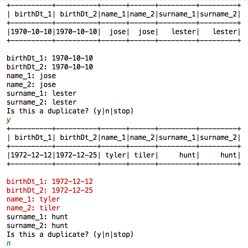
The labeling takes the form of a console application that iteratively displays a potential duplicate and queries the human for a decision:

Predictions

Then comes the time where we can train the Machine Learning algorithm. We chose to use Spark ML’s Random Forests classifier as they do a pretty good job, but Gradient Boosting Trees would have been another valid option.

The training is done on the potential duplicates that have been labeled by hand. We used 80% of the dataset as the training set and the remaining 20% as the test set. As a reminder, this allows the evaluation of the model to be performed on a different dataset than the training one, and thus prevents from overfitting.

Once the model is ready, we can apply it on the potential duplicates that have not been labeled by hand.

Let’s have a quick look at the accuracy of the model. When training the model on a sample of 1000 records (i.e. 200 records in the test set), we found the following results:

True positives: 53
False positives: 2
True negatives: 126
False negatives: 5

True positives and true negatives are records for which we predicted the correct – true or false – answer. False positives and false negatives are errors.

A good way to evaluate the relevance of the predictions is to calculate the precision and recall scores. The precision determines how many selected items are relevant, while the recall indicates how many relevant items are selected. In our case, precision is 93% and recall is 91%. That’s not bad and, in fact, that’s much better than what was previously achieved with a naïve implementation (around 50%).

Summary & Conclusion

To summarize, we have implemented an engine that allows us to do Record Linkage and Deduplication with the same code. Instead of using fixed rules to find duplicates, we used a Machine Learning algorithm that adapts to each dataset.

The data processing was implemented using Spark and more precisely DataFrames. DataFrames are handy in this use case because they can carry an arbitrary number of columns.

For the Machine Learning, we used Spark ML, the Machine Learning library that works on top of DataFrames. While the Machine Learning part is often what scares developers, it was in the end easier to implement than the data processing itself.

We are quite happy with this application as it gives a higher identification of matches: between 80 and 90% while we were only reaching 50% with another method.

Record Linkage, a real use case with Spark ML